Homework10

GGPlots

library(ggplot2) # for graphics
library(tidyverse)
library(tidytuesdayR) # for data set
library(ggridges) # for ridges
library(dplyr)
library(tidyr)
library(ggbeeswarm)
library(beeswarm)
library(ggridges)

Calling in Datasets

This calls in our data set and assign it a name

tuesdata <- tidytuesdayR::tt_load('2024-04-23')
outer_space_objects <- tuesdata$outer_space_objects

Properly Filtered data

# Filtered Data set 1
filtered_data <- outer_space_objects %>%
  filter(Entity %in% c("Canada", "Brazil", "China", "Denmark","Argentina","Chile","Colombia","Finland","France","Germany"))
colnames(filtered_data) <- c("Country","Code","Year","satellite")

# Filtered Data Set 2
filtered_data2 <- outer_space_objects %>%
  filter(Entity %in% c("Canada", "Brazil", "China"))
colnames(filtered_data2) <- c("Country","Code","Year","satellite")

# Filtered Data Set 3
filtered_data3 <- outer_space_objects %>%
  filter(Entity %in% c("Canada", "Brazil", "Germany","Denmark"))
colnames(filtered_data3) <- c("Country","Code","Year","satellite")

Ridgeline Graph

p2 <- ggplot(data=filtered_data) +
  aes(x=Year,y=Country,fill=Country) +
  ggridges::geom_density_ridges() +
  ggridges::theme_ridges(font_size = 14,
                         font_family = "Times New Roman",
                         line_size = 0.5,
                         grid = TRUE,
                         center_axis_labels = FALSE)
p2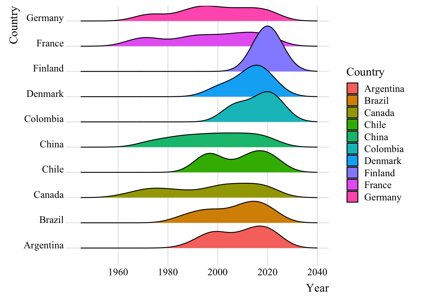

Bee Swarm Graph

p3 <- ggplot(data=filtered_data2) +
  aes(x=Country,y=satellite,color=Country) +
  ggbeeswarm::geom_beeswarm(method = "center",size=1.5) +
  scale_color_manual(values = c(
    "Canada" = "cornflowerblue",
    "Brazil" = "darkolivegreen3",
    "China" = "darkred"
  )) +
  ggridges::theme_ridges(font_size = 14,
                         font_family = "Times",
                         line_size = 0.3,
                         grid = TRUE,
                         center_axis_labels = FALSE)
# The code above creates the graph

p3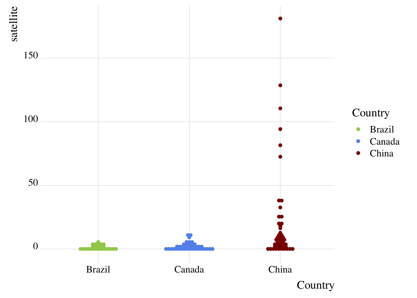

Waffle Graph

p8 <- ggplot(data=filtered_data3) +
  aes(fill = Country, values = satellite) +
  ggtitle("    Number of individuals Satellites Sent to Space") +
  waffle::geom_waffle(n_rows = 8, size = 0.33, colour = "white") +
  coord_equal() +
  theme_void()

p8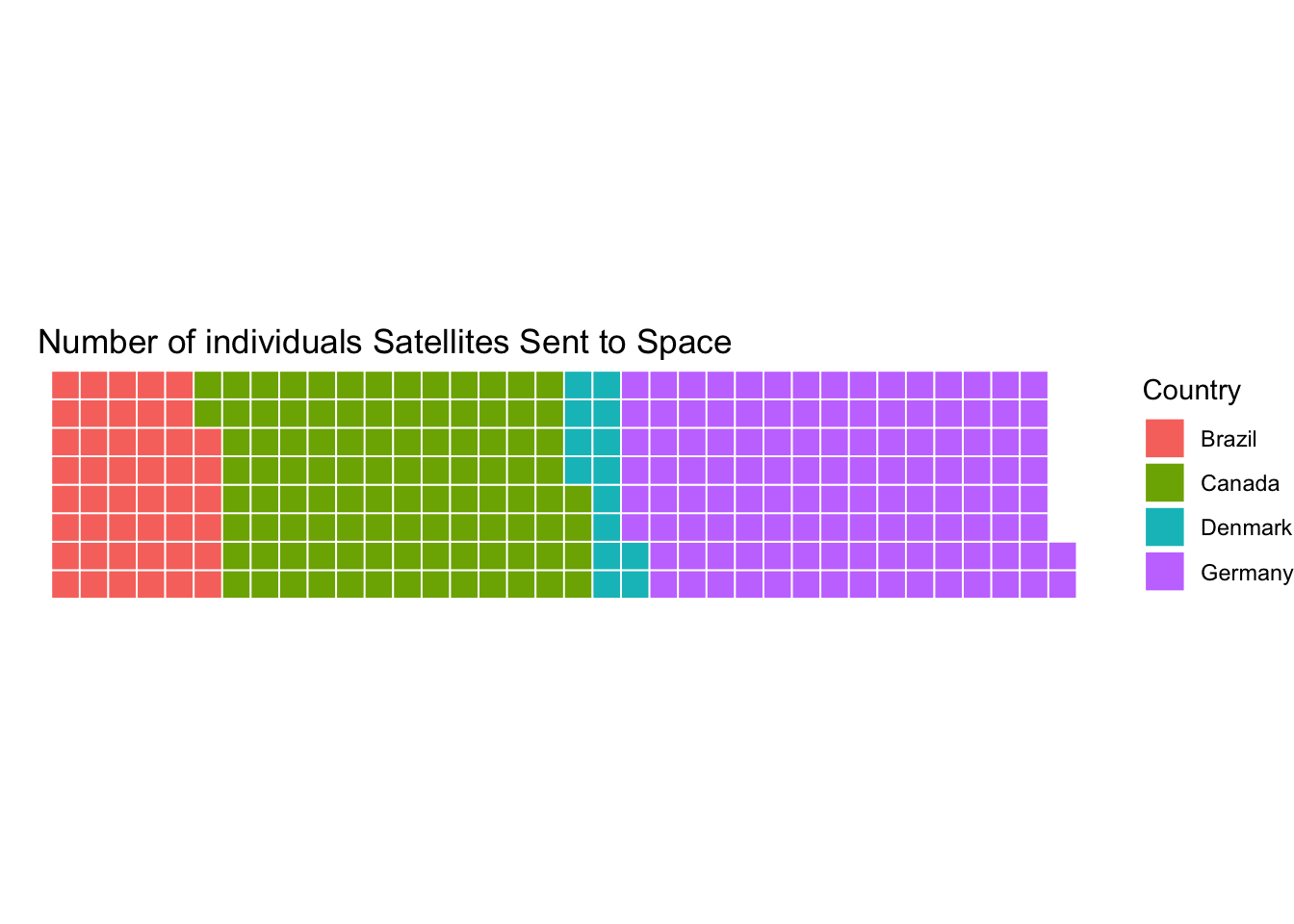

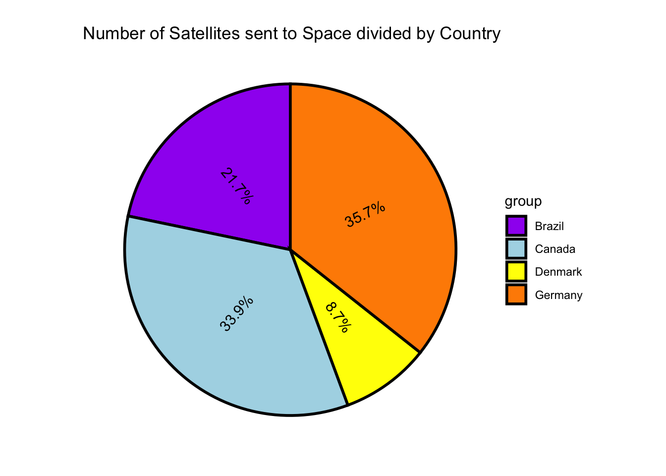
Horrible Pie Graph

p5 <- ggpie::ggpie(data=filtered_data3,
                   group_key="Country",
                   count_type="full",
                   label_info="ratio",
                   label_type="circle") +
    ggtitle("Number of Satellites sent to Space divided by Country") +
  scale_fill_manual(values = c("purple", "lightblue", "yellow", "darkorange"))

p5